The circuit
In this example the fifth-order active low-pass filter will be optimised by optimize command. The circuit is shown in figure below.
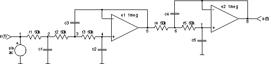
We can see, that we have two ideal operational amplifiers with 120dB gain and five resistors and capacitors, which determine pole locations in s plane. In fact all circuit poles can be set without changing resistor values. So all resistors are the same (resistance is 50kW).
Here is the netlist of the circuit (part of
fifth-order_active_low-pass_filter.cir file):
*** the fifth-order low-pass filter ***

vin 1 0 dc 0 ac 1V

r1 1 2 50k
r2 2 3 50k
r3 3 4 50k
r4 5 6 50k
r5 6 7 50k

c1 2 0 250nF
c2 4 0 25nF
c3 3 5 500nF
c4 6 8 500nF
c5 7 0 5nF

e1 5 0 4 5 1meg
e2 8 0 7 8 1meg

.end
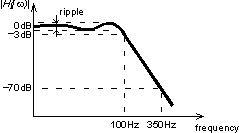
We want to design the low-pass filter with -3dB at 100Hz (cutoff frequency) and at least -70dB at 350Hz. Minimal ripple is desired at the same time. So we are looking for capacitances c1, c2, c3, c4 and c5, which will give the most satisfying frequency response. Frequency response is in our case given by:
H(j w) = H(jw, c1, c2, c3, c4, c5)
Because of the given circuit topology the dc gain will always be 0dB for arbitrary capacitances c1, c2, c3, c4 and c5.
H(j0, c1, c2, c3, c4, c5) = 1 = 0dB
We can estimate the explicit constraints of the capacitances c1, c2, c3, c4 and c5.
50nF < c1 < 500nF
5nF < c2 < 50nF
100nF < c3 < 1uF
100nF < c4 < 1uF
1nF < c5 < 10nF
In this example, we are searching for the capacitances c1, c2, c3, c4 and c5 inside these intervals, which will give the required frequency response.
Now we have to define the cost function. It has to increase with ripple, difference between cutoff frequency and 100Hz and dBs above -70dB at 350Hz. The cost function will be defined by simply adding those three requests without weights (all are equally important). The second request will not be strictly realised. The cost function will be increased if frequency response is below -3dB at 98Hz (cutoff frequency is to low) and if frequency response is above -3dB at 102Hz (cutoff frequency is to high).
E(c1, c2, c3, c4, c5) = (ripple) +
((below -3dB at 98Hz) + (above -3dB at 102Hz)) +
(above -70dB at 350Hz)
Because we are interested only in vector
v(8), we will not save all other vectors calculated in a particular analysis.
save command defines which vectors will be saved. Then the circuit's netlist is loaded by
source command.
Spice Opus 1 -> source (filename with netlist of the circuit)
Circuit: *** the fifth-order low-pass filter ***
Spice Opus 2 -> save v(8)
First we have to define the parameters, which can vary in the optimisation process. Those are
capacitances of elements
c1,
c2,
c3,
c4 and
c5. This can be done by
optimize parameter command. At the same time we will give the explicit constraints for all parameters and the initial point
(c1 = 250nF,
c2 = 25nF,
c3 = 500nF,
c4 = 500nF and
c5 = 5nF), where the optimisation algorithm will start.
Spice Opus 3 -> optimize parameter 0 @c1[capacitance]
  low 50n high 500n initial 250n
Spice Opus 4 -> optimize parameter 1 @c2[capacitance]
  low 5n high 50n initial 25n
Spice Opus 5 -> optimize parameter 2 @c3[capacitance]
  low 100n high 1u initial 500n
Spice Opus 6 -> optimize parameter 3 @c4[capacitance]
  low 100n high 1u initial 500n
Spice Opus 7 -> optimize parameter 4 @c5[capacitance]
  low 1n high 10n initial 5n
We also have to define the commands, which will be executed in every iteration. Those commands have to provide data for computing the value of the cost function and for verifying the implicit constraints (in this example there are no implicit constraints). To compute the cost function the frequency response is needed. It will be computed by three
ac analyses, so we will define three
ac commands by
optimize analysis command.
Spice Opus 8 -> optimize analysis 0 ac lin 100 10Hz 95Hz
Spice Opus 9 -> optimize analysis 1 ac lin 3 98Hz 102Hz
Spice Opus 10 -> optimize analysis 2 ac lin 3 350Hz 360Hz
The expression for the cost function have to be defined next. We will use the optimize cost command. The expression have to be written in standard Nutmeg language.
Spice Opus 11 -> optimize cost max(db(ac1.v(8))) - min(db(ac1.v(8))) +
  (db(ac2.v(8)[0]) lt -3) * abs(db(ac2.v(8)[0]) + 3) +
  (db(ac2.v(8)[2]) gt -3) * (db(ac2.v(8)[2]) + 3) +
  (db(ac3.v(8)[0]) gt -70) * (db(ac3.v(8)[0]) + 70)
The optimisation method and its parameters can be defined by
optimize method command. We will choose the constrained simplex method
(complex) with default settings.
Spice Opus 12 -> optimize method complex
Now we are ready to start the optimisation algorithm by
optimize command without parameters. When the algorithm converges the results and some statistics are written.
Spice Opus 13 -> optimize
Complex: stopped, simplex small enough
Time needed for optimisation: 7.869 seconds
Number of iterations: 565
Lowest cost function value: 5.920833e-001
Optimal values:
@c1[capacitance]	=	1.105419e-007
@c2[capacitance]	=	9.081350e-009
@c3[capacitance]	=	2.275500e-007
@c4[capacitance]	=	3.103057e-007
@c5[capacitance]	=	3.384043e-009
It is interesting to see how did the parameter values (capacitances) travel around the parameter space during the optimisation. The normalised values of the capacitances can be plotted by
plot command.
Spice Opus 14 -> plot (c1_capacitance-5e-8)/45e-8
  (c2_capacitance-5e-9)/45e-9 (c3_capacitance-1e-7)/9e-7
  (c4_capacitance-1e-7)/9e-7 (c5_capacitance-1e-9)/9e-9
  xlabel iteration ylabel capacitances
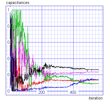
We can see that rough optimal values are determined after 350 iterations.
We optimised our low-pass filter. Now we will determine capacitances analytically and compare them with obtained results. The fifth-order 0.5dB Chebyshev low-pass filter meet our requirements. We can calculate the capacitances and compare them:
| analytic | optimised | ||
| c1 | 106nF | 111nF | |
| c2 | 9.66nF | 9.08nF | |
| c3 | 218nF | 228nF | |
| c4 | 301nF | 310nF | |
| c5 | 3.64nF | 3.38nF |
| pole | analytic | optimised | |
| 1. | -214 | -201 | |
| 2. | -174 - j371 | -167 - j381 | |
| 3. | -174 + j371 | -167 + j381 | |
| 4. | -66.4 - j601 | -66.5 - j614 | |
| 5. | -66.4 + j601 | -66.5 + j614 |
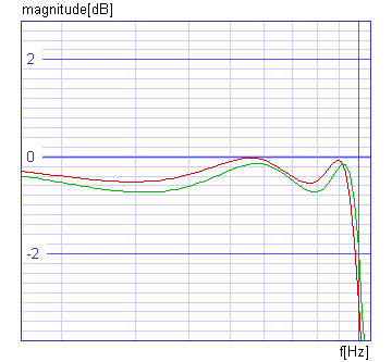
Finally it is interesting to compare frequency responses of optimised and analytic filter. Capacitances will be changed to analytically calculated by
alter command.
Spice Opus 15 -> ac dec 100 1Hz 1kHz
Spice Opus 16 -> alter c1 capacitance = 106n
Spice Opus 17 -> alter c2 capacitance = 9.66n
Spice Opus 18 -> alter c3 capacitance = 218n
Spice Opus 19 -> alter c4 capacitance = 301n
Spice Opus 20 -> alter c5 capacitance = 3.64n
Spice Opus 21 -> ac dec 100 1Hz 1kHz
Spice Opus 22 -> plot db(ac1.v(8)) db(ac2.v(8))
  xlabel f[Hz] ylabel magnitude[dB] title 'AC analyses'

Spice Opus 23 -> _
We can see that the filters are almost identical and that they equally satisfy our requirements.
The input file (fifth-order_active_low-pass_filter.cir) comes with the installation. It does not do exactly the same steps which are described above.